Goal - Estimate the relative transmissivity change or head
Transmissivity solution
Given (Sokol eq 6): The example will be a single unit where we add a new one.
\[h_w = \frac{T_1 H_1}{T_1}\] \[h_w + \Delta h_w = \frac{T_1 H_1 + T_2 H_2}{T_1 + T_2}\]
where:
- \(h_w\) is the blended head for the shorter interval
- \(h_w + \Delta h_w\) is the blended head for the larger interval
- \(T_1\) is the transmissivity for the shorter interval
- \(T_1 + T_2\) is the transmissivity for the larger interval
- \(H_2\) is the head corresponding to the \(T_2\) interval
Multiply denominators:
\[h_w T_1 = T_1 H_1\] \[h_w T_1 + h_w T_2 + \Delta h_w T_1 + \Delta h_w T_2 = T_1 H_1 + T_2 H_2\]
Subtract first from second:
\[h_w T_2 + \Delta h_w T_1 + \Delta h_w T_2 = T_2 H_2\]
Put \(T_2\) on one side: \[\Delta h_w T_1 = T_2 H_2 - h_w T_2 - \Delta h_w T_2\]
Rearrange: \[\frac{\Delta h_w T_1}{H_2 - h_w - \Delta h_w} = T_2\]
Can also solve for the transmissivity ratio: \[\frac{\Delta h_w}{H_2 - h_w - \Delta h_w} = \frac{T_2}{T_1}\]
Examples
Can we recover missing values? In this example we test if we can recover the missing value for the \(10^{th}\) interval.
library(sokol)

set.seed(123)
transmissivity <- abs(rnorm(10))
head <- sort(rnorm(10))
plot_blended(transmissivity, head)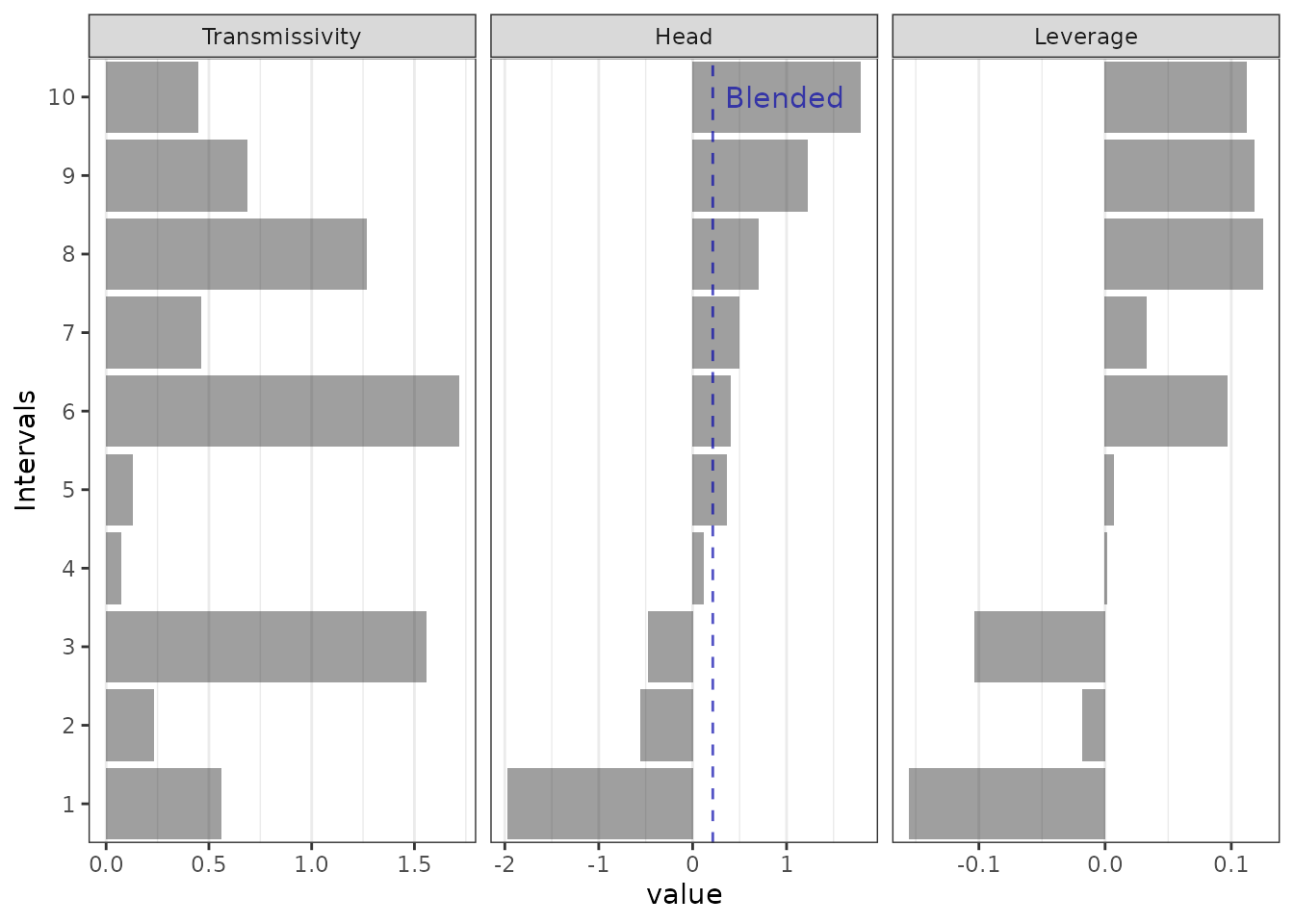
blended_1 <- estimate_blended_head(transmissivity[1:9], head[1:9])
blended_2 <- estimate_blended_head(transmissivity, head)


# estimate interval head
estimate_missing(blended_2,
                 c(transmissivity),
                 c(head[1:9], NA_real_))
#> [1] 1.786913
head[10]
#> [1] 1.786913


# estimate interval transmissivity
estimate_missing(blended_2,
                 c(transmissivity[1:9], NA_real_),
                 c(head))
#> [1] 0.445662
transmissivity[10]
#> [1] 0.445662


# estimate blended head
estimate_missing(NA_real_,
                 c(transmissivity),
                 c(head))
#> [1] 0.2145803
blended_2
#> [1] 0.2145803