Introduction

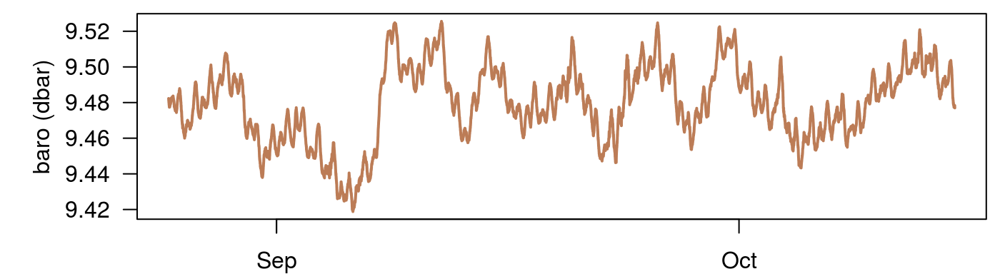
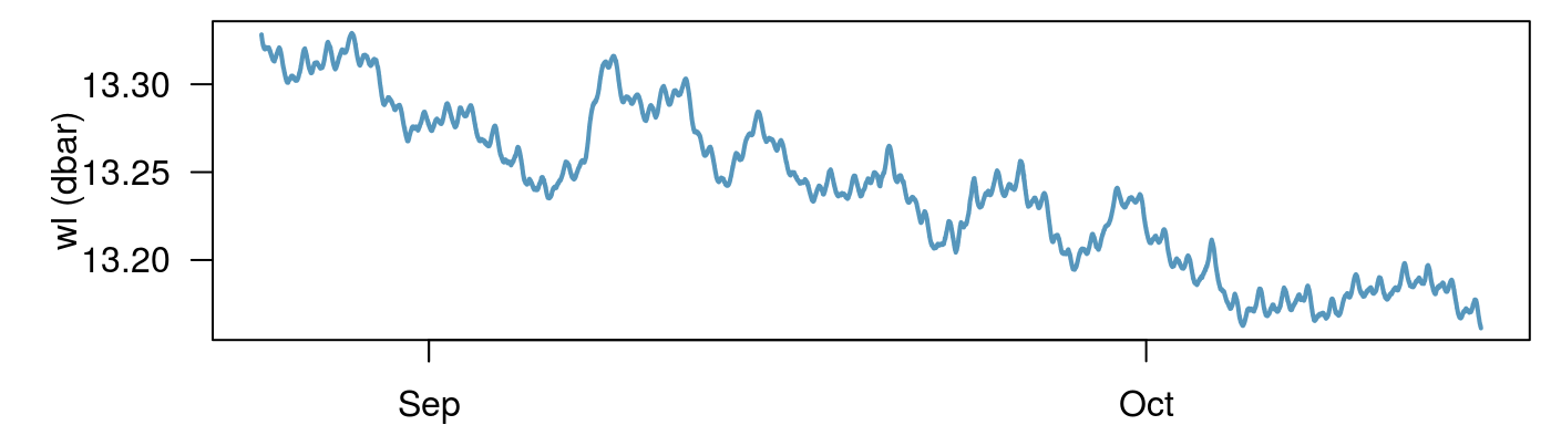
This vignette covers the static barometric/loading efficiency (BE/LE) calculations in the waterlevels package. We will use a dataset collected from a fractured sandstone site (called transducer) as an example which has 1.5 month of data collected every 2 minutes and columns called datetime, wl, et, and baro which corresponds to the date and time of the analysis, the water level pressure from a non-vented submerged transducer, the synthetic Earth tide, and the atmospheric pressure from a non-vented transducer. We use the raw pressure measurements and the raw barometric pressure data (i.e. there is no reason to convert to an estimated water level for these analyses).

Static barometric efficiency calculations are simple to apply but it is important to consider their applicability on a well by well basis.

In particular, these methods assume:

That there is no time-lag in the response between the water levels and the barometric pressure. This response is often called the fully confined response. If the monitoring frequency is large in comparison to the time lag this assumption may be relaxed somewhat.

We start by loading the packages and applicable data for the loading efficiency calculation.

First step: Plot the data

Remove a trend

It is often important to remove trends from the data prior to analysis. We will remove the trend in the water level data and the barometric pressure data using linear regression. Some methods are more robust for handling data with complicated trends, but for this dataset, and these analyses a linear trend should suffice. We can then replot the values. Now that we have removed the trend we can plot the water level pressure and the atmospheric pressure on the same figure for coparison.

data(transducer)
transducer[, wl_detrend := lm(wl~datetime)$residuals]
transducer[, baro_detrend := lm(baro~datetime)$residuals]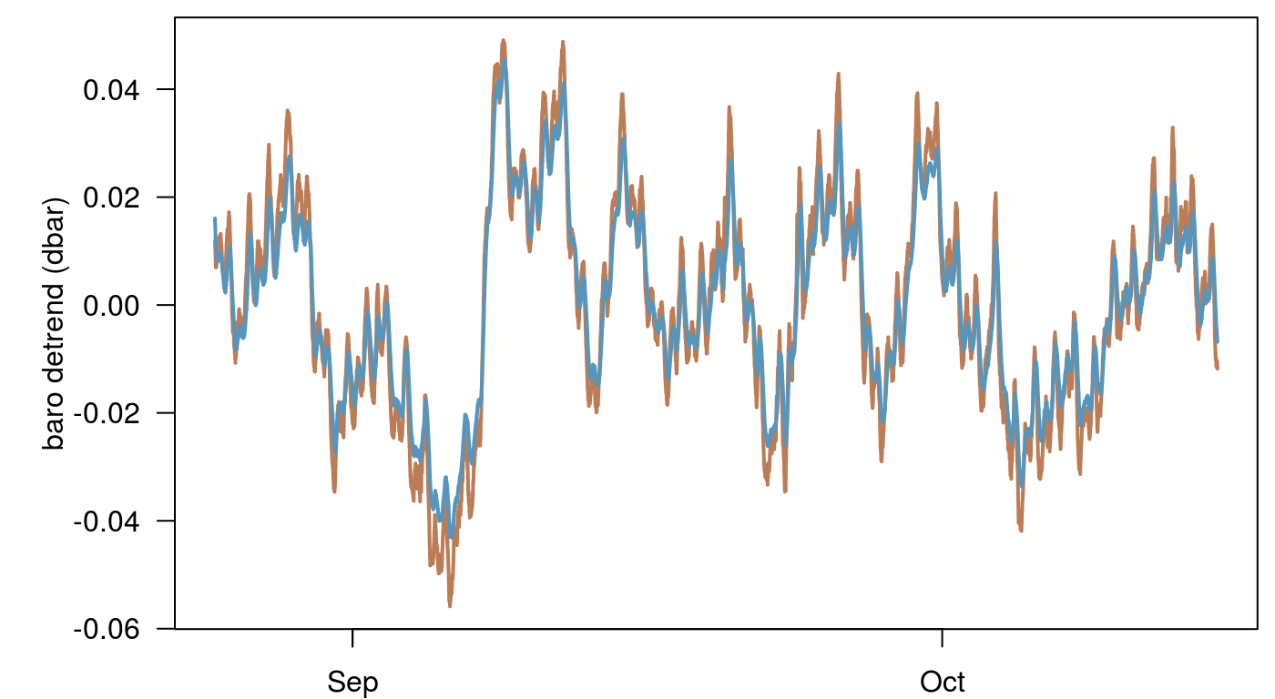

The two responses look very similar. At this scale it appears that the water level response is a smoothed version of the barometric response with a slightly diminished magnitude. Let’s explore this more fully.

Calculate Barometric/Loading Efficiency

There are many ways to calculate the barometric/loading efficiency. I have tried to include as many methods as possible in the waterlevel package and if you know of a method I missed let me know and I will do my best to add it.

Least squares

This method is just a simple wrapper for least squares regression added to be consistent with the other functions in the package. The inverse column is either TRUE or FALSE and deserves a few words here. The value should be set to TRUE to signify that if the independent variable (atmospheric pressure) increases the dependent variable decreases (dep). This is typically the case for vented transducers and water level obtained via a water level tape. The result of this calculation will be a barometric efficiency. For non-vented transducers when atmospheric pressure increases the submerge pressure reading also increases. The result of this calculation is the loading efficiency.

Summary:

Loading efficiency, when inverse == FALSE (for non-vented transducers)
Barometric efficiency, when inverse == TRUE (for vented transducers, manual measurements)

be_ls <- be_least_squares(dat = transducer, 
                          dep = 'wl_detrend', 
                          ind = 'baro_detrend',
                          inverse = FALSE,
                          return_model = FALSE)

# This value is the BE/LE
be_ls
#> [1] 0.827616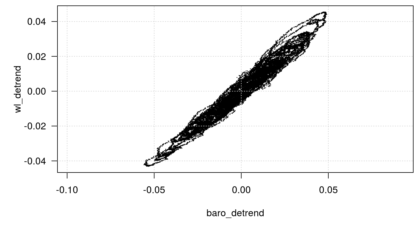

If you are interested in the residuals from the model fit or the regression results you may specify return_model = TRUE. In this method the loading efficiency is 0.83.

Least squares using first differences

In the presence of background trends running the regression on first differences can minimize their effect on the regression results. To apply this method we have one more parameter called lag_space which determines how many samples are between difference calculations. This value is important when monitoring frequency is high. Commonly BE/LE calculates the differences based on data collected at 1 hour increments. So for this example where we collected 2 minute data that translates to a lag_space of 30

be_lsd <- be_least_squares_diff(dat = transducer, 
                                dep = 'wl_detrend', 
                                ind = 'baro_detrend',
                                lag_space = 30,
                                inverse = FALSE,
                                return_model = FALSE)

# This value is the BE/LE
be_lsd
#> [1] 0.4475877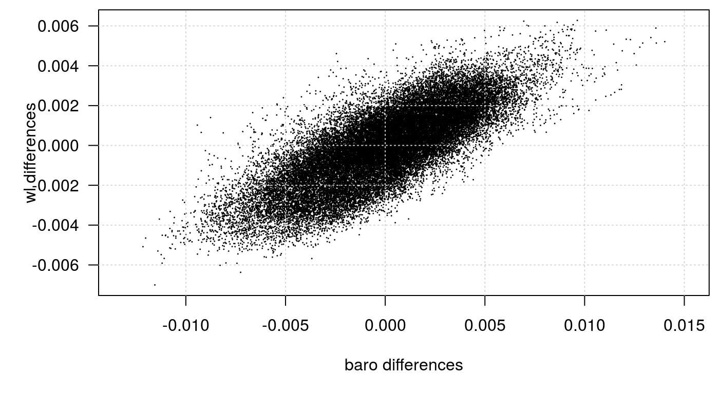

The least squares value of 0.83 is not very similar least squares differences method of 0.45. Why might this be? What happens if we change the difference_space value?

# test 1 to 2880 lag_space
difference_spaces <- 2^(0:13)

be_lsds <- sapply(difference_spaces, function(x) {
  be_least_squares_diff(dat = transducer, 
                        dep = 'wl_detrend', 
                        ind = 'baro_detrend',
                        lag_space = x,
                        inverse = FALSE,
                        return_model = FALSE)
})

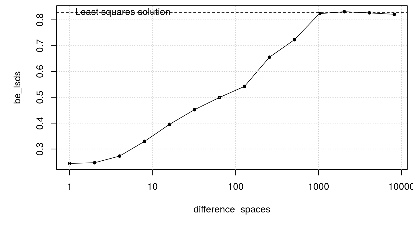
So by using a different lag_space we can get agreement between the two methods. Let’s see how other methods perform.

Clark (1967)

This function has the same arguments as be_least_squares_diff. This method will likely suffer from a similar problem as we saw with be_least_squares_diff. Let’s use differences of 1 day as this appeared to give consistent results to the original least squares method.

be_c <- be_clark(dat = transducer, 
                 dep = 'wl_detrend', 
                 ind = 'baro_detrend',
                 lag_space = 720,
                 inverse = FALSE,
                 return_model = FALSE)

be_c
#> [1] 0.8524435

Rahi and Halihan (2013)

The Rahi method is similar to the Clark method but has a magnitude check in addition to the sign check that Clark’s method does. The arguments are the same for the current implementation except we do not have a return_model option.

be_r <- be_rahi(dat = transducer, 
                dep = 'wl_detrend', 
                ind = 'baro_detrend',
                lag_space = 720,
                inverse = FALSE)

be_r
#> [1] 0.8068093

Ratio method (Gonthier 2007)

This method calculates the ratio for each difference. Then filters them based on the magnitude of the barometric pressure change (quant), and finally summarizes the data using stat. We will calculate the one-day differences, select those having the largest barometric pressure changes (top 10 percentile), and take the median of the resulting ratios.

be_rat <- be_ratio(dat = transducer, 
                   dep = 'wl_detrend', 
                   ind = 'baro_detrend',
                   lag_space = 720,
                   quant = 0.9,
                   stat = median,
                   inverse = FALSE)
be_rat
#> [1] 0.8305719

High-low method

The high-low method compares water level changes to barometric pressure changes for different time periods. We specify the column name that holds the time and a time_group which is the size of the time interval in seconds. Here we calculate the LE every day for our dataset. This method will tend to overestimate the BE/LE.

be_hl <- be_high_low(dat = transducer, 
                     dep = 'wl_detrend', 
                     ind = 'baro_detrend',
                     time = 'datetime',
                     time_group = 86400*7)

head(be_hl)
#>         start                 end    diff_wl  diff_baro    n     ratio
#> 1: 2016-08-25 2016-08-31 23:58:00 0.05493151 0.07071531 5040 0.7767980
#> 2: 2016-09-01 2016-09-07 23:58:00 0.06159079 0.07435261 5040 0.8283609
#> 3: 2016-09-08 2016-09-14 23:58:00 0.06041294 0.06903326 5040 0.8751280
#> 4: 2016-09-15 2016-09-21 23:58:00 0.04990858 0.06869495 5040 0.7265248
#> 5: 2016-09-22 2016-09-28 23:58:00 0.05999510 0.07749294 5040 0.7742008
#> 6: 2016-09-29 2016-10-05 23:58:00 0.06364050 0.08117460 5040 0.7839952

Smith, van der Kamp, and Hendry (2013)

I like this method for data where there is a complex trend. It uses informed judgement to fit the best BE/LE value. We supply different values of BE which are then used to remove the barometric signal from the data. The goal is to have a smooth curve (or a result that matches our expectations) after the barometric pressure is removed.


be_visual(transducer[seq(1, nrow(transducer), 90)],
          dep = 'wl_detrend',
          ind = 'baro_detrend',
          time = 'datetime',
          be_tests = seq(0.6, 1.0, 0.05),
          inverse = FALSE,
          subsample = TRUE)

What value do you estimate for LE? How certain are you? Why is there stucture in the residuals? One reason is that this data is from a semi-confined well with non-negligible well-bore storage and we have violated the assumption that there is no time lag in the response. A better technique for this well would have been to use barometric/loading response functions.

Acworth method

Acworth and Brain (2008)

Acworth et al. (2016)

Acworth et al. (2017)

G. C. Rau et al. (2018)]

This method uses frequency domain values and includes the Earth tide response. The BE/LE is calculated by using ratio of the barometric pressure harmonic (S₂) and the water level harmonic (S₂) corrected for Earth tides. It is meant to be applied to confined wells. This value is also tied to the semi-diurnal frequency and care needs to be taken on it’s interpretation in the same way the time based static barometric efficiency calculations are limited. See the response function vignette for a more complete view of the water level response.

be_a <- be_acworth(transducer, wl = 'wl', ba = 'baro', et = 'et', 
                   inverse = FALSE)

be_a
#> [1] 0.5793122

References

Acworth, R. I., and T. Brain. 2008. “Calculation of barometric efficiency in shallow piezometers using water levels, atmospheric and earth tide data.” Hydrogeology Journal 16 (8). Springer-Verlag: 1469–81. doi:10.1007/s10040-008-0333-y.

Acworth, R. I., L. J. Halloran, G. C. Rau, M. O. Cuthbert, and T. L. Bernardi. 2016. “An objective frequency domain method for quantifying confined aquifer compressible storage using Earth and atmospheric tides.” Geophysical Research Letters 43 (22). John Wiley & Sons, Ltd: 11, 671–11, 678. doi:10.1002/2016GL071328.

Acworth, R. I., G. C. Rau, L. J. Halloran, and W. A. Timms. 2017. “Vertical groundwater storage properties and changes in confinement determined using hydraulic head response to atmospheric tides.” Water Resources Research 53 (4). John Wiley & Sons, Ltd: 2983–97. doi:10.1002/2016WR020311.

Clark, W. E. 1967. “Computing the Barometric Efficiency of a Well.” Journal of the Hydraulics Division 93 (4). ASCE: 93–98.

Gonthier, G. J. 2007. “A Graphical Method for Estimation of Barometric Efficiency from Continuous Data–concepts and Application to a Site in the Piedmont.” Air Force Plant 6.

Rahi, K. A., and T. Halihan. 2013. “Identifying aquifer type in fractured rock aquifers using harmonic analysis.” GroundWater 51 (1). John Wiley & Sons, Ltd (10.1111): 76–82. doi:10.1111/j.1745-6584.2012.00925.x.

Rau, G. C.., R. I. Acworth, L. J. S. Halloran, W. A. Timms, and M. O. Cuthbert. 2018. “Quantifying Compressible Groundwater Storage by Combining Cross-Hole Seismic Surveys and Head Response to Atmospheric Tides.” Journal of Geophysical Research: Earth Surface 123 (8). John Wiley & Sons, Ltd: 1910–30. doi:10.1029/2018JF004660.

Smith, L. A., G. van der Kamp, and J. M. Hendry. 2013. “A new technique for obtaining high-resolution pore pressure records in thick claystone aquitards and its use to determine in situ compressibility.” Water Resources Research 49 (2): 732–43. doi:10.1002/wrcr.20084.

Static Barometric/Loading Efficiency Calculations

2019-05-13