Introduction

To test the efficiency of different methods we will create a response function, apply it to some barometric pressure data to generate a synthetic water level response.

Response function

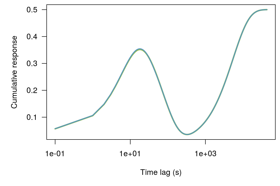
This is the function we will try to recreate! It is the combination of three exponentials of different lengths:

60 second (negative)
600 second (negative)
43201 second (positive)

exp1 <- -exp(-seq(0.01, 8, length.out = 60))
exp2 <- -exp(-seq(0.01, 8, length.out = 43201))
exp3 <- exp(-seq(0.01, 8, length.out = 600))

exp1 <- exp1 /  sum(exp1)
exp2 <- exp2 /  sum(exp2)
exp3 <- exp3 / -sum(exp3)

exp1 <- c(exp1, rep(0.0, length(exp2) - length(exp1)))
exp3 <- c(exp3, rep(0.0, length(exp2) - length(exp3)))
kern <- rev(exp1 + exp2 + exp3)

resp_fun <- cumsum(rev(kern))*0.5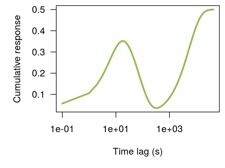

Barometric pressure

We can get a barometric response with the synthetic function.

Synthetic water levels

Convolution of barometric pressure data and response function. Water levels have a dampened appearance and are lagged slightly in relation to the barometric response. This is commonly observed at field sites. There is no noise in this example so we hope to perfectly recover the response function.

dat <- synthetic(sd_noise = 0e-2,
                 sd_noise_trend = 0e-12,
                 n = 4 * 86400,
                 linear_trend = 0e-12,
                 seed = 1,
                 baro_kernel = kern)[, list(datetime, baro, wl)]

dat <- dat[1:(2.5 * 86400)]
dat[, baro := baro - mean(baro, na.rm = TRUE)]
dat[, wl := wl - mean(wl, na.rm = TRUE)]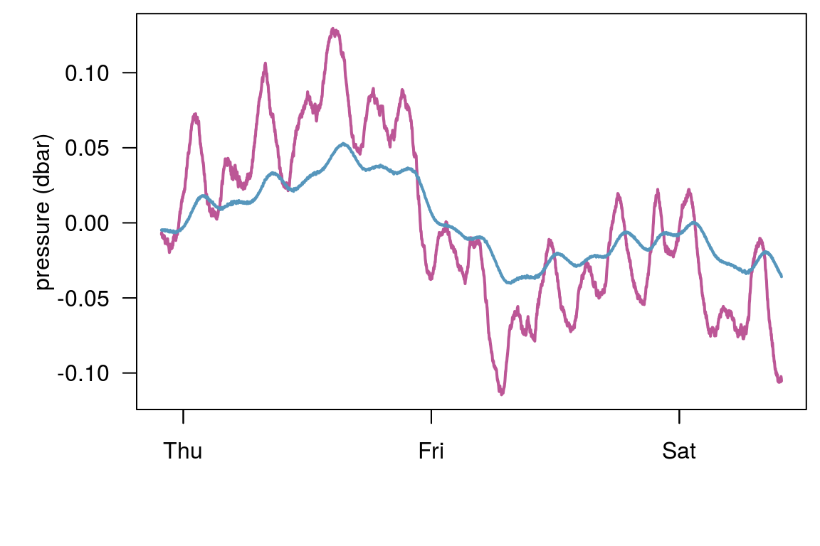

Regular lag method

Regular lag methods can generate large regression matrices, and therefore, we will subset our data prior to analysis. We start with one second data, but will subset to 60 seconds. The matrix size will be

dt <- 60

dat_sub <- dat[seq(1, nrow(dat), dt)]

ba_lags <- seq(0, (43200+dt) / dt, 1)

rec <- recipe(wl~., dat_sub) %>%                          
  step_lag_matrix(baro, lag = ba_lags) %>%                   
  prep() %>%                                                
  portion()

dim(rec)
#> [1] 3600    3

Do regression

What if we only had data every 30 minutes?

#>    n_obs n_coef   df        sigma r_squared       AIC       BIC   logLik
#> 1:  2879    723 2156 5.316373e-05  0.999997 -47885.33 -43566.53 24666.67

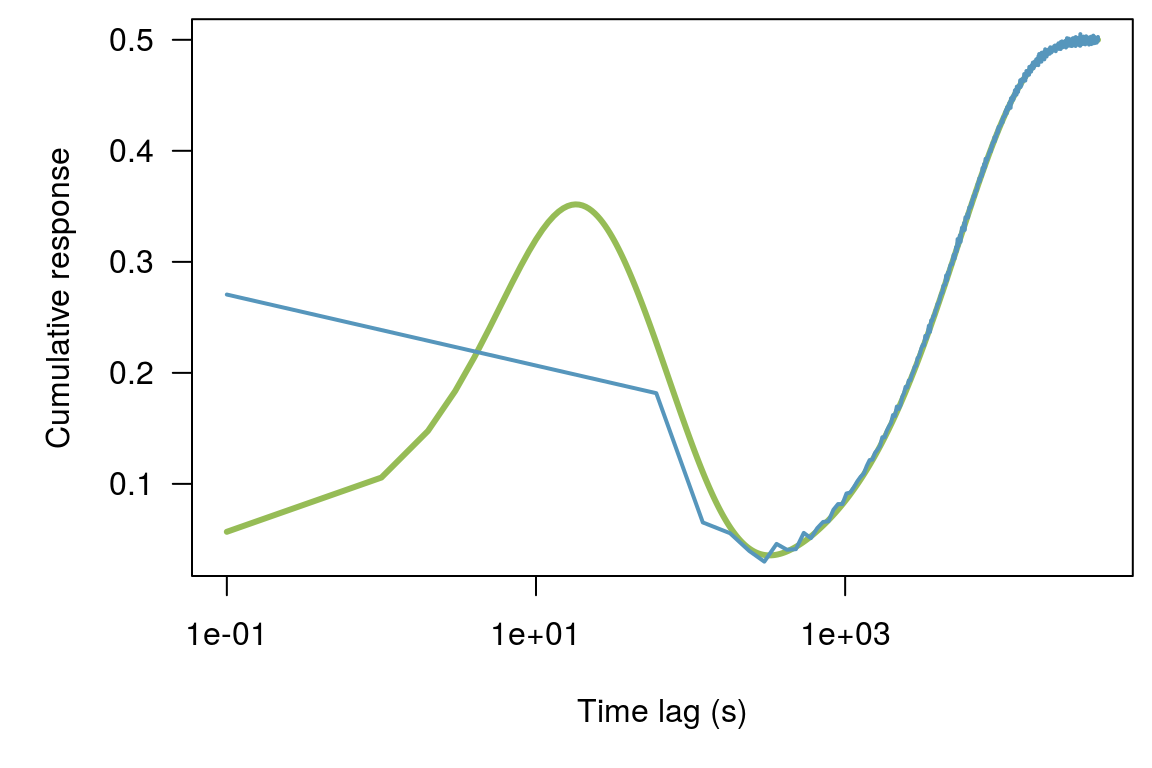
Irregular lag method

We won’t subset in this case. We will use fewer regressors but have many more observations. These results are even better.

ba_lags <- log_lags(251, max_time_lag = 43201)

rec <- recipe(wl~., dat) %>%                          
  step_lag_matrix(baro, lag = ba_lags) %>%                   
  prep() %>%                                                
  portion()

dim(rec)
#> [1] 216000      3

#>     n_obs n_coef     df        sigma r_squared      AIC      BIC  logLik
#> 1: 172800    201 172599 2.341373e-05 0.9999992 -3194264 -3192232 1597334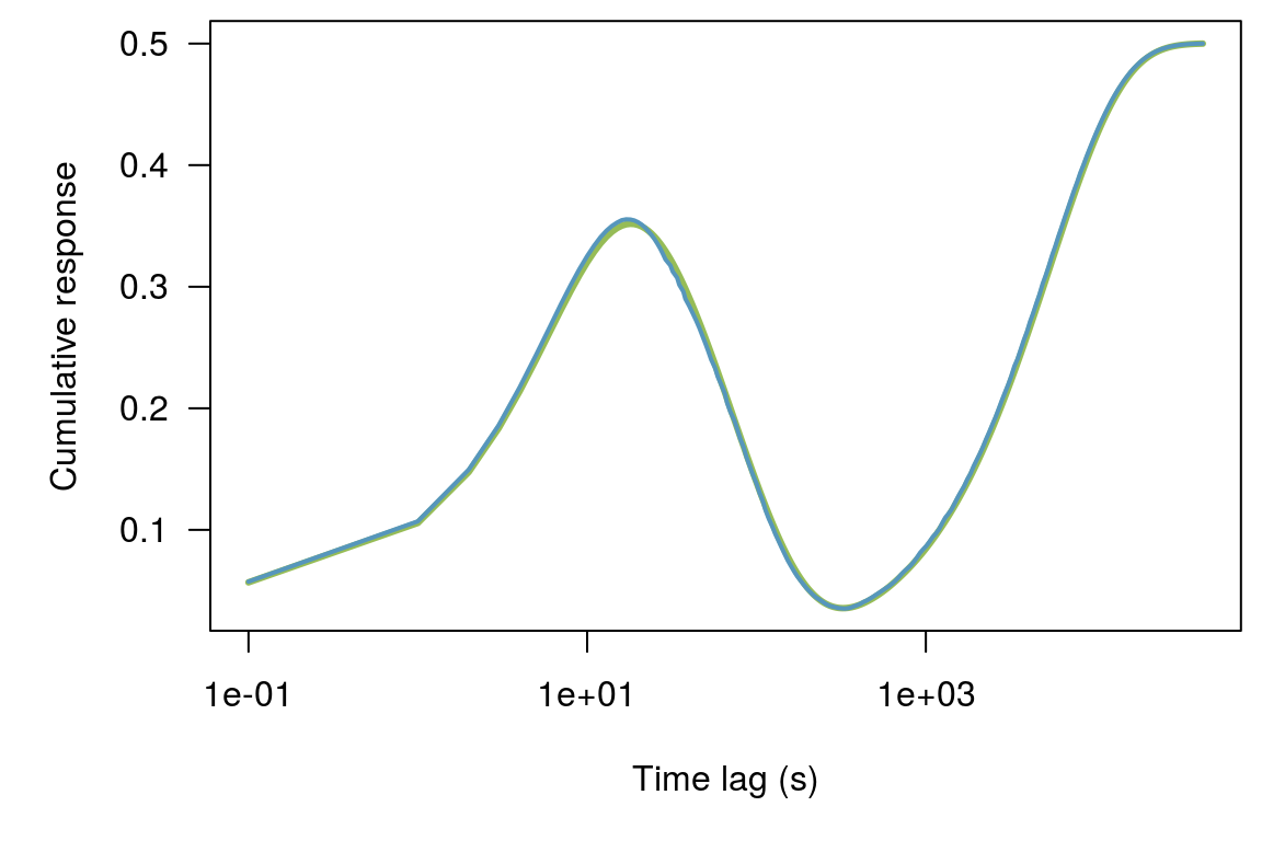

Distributed lag method

We won’t subset in this case and we will only use 15 regressors.

ba_lags <- log_lags(18, max_time_lag = 43201)

rec <- recipe(wl~., dat) %>%                          
  step_distributed_lag(baro, knots = ba_lags) %>%                   
  prep() %>%                                                
  portion()

dim(rec)
#> [1] 216000      3

#>     n_obs n_coef     df        sigma r_squared      AIC      BIC  logLik
#> 1: 172800     19 172781 5.672424e-06         1 -3684405 -3684204 1842223

Synthetic example

2019-05-13