Aquifer steps
aquifer.RmdGeneralized radial flow model (Barker, 1988)
time <- as.numeric(1:2000)
flow_rate <- c(rep(0.001, 500),
                rep(0.002, 500),
                rep(0.0, 1000))

# radial (flow_dimension = 2 Theis)
dat <- data.frame(time = time,
                  flow_rate = flow_rate)
formula <- as.formula(flow_rate~time)
grf = recipe(formula = formula, data = dat) |>
  step_aquifer_grf(time = time,
                   flow_rate = flow_rate,
                   thickness = 1.0,
                   radius = 20.0,
                   specific_storage = 1e-5,
                   hydraulic_conductivity = 1e-3,
                   flow_dimension = 2) |>
  plate()
#> a: 0


plot(aquifer_grf~time, grf,
     type = "l",
     ylab = "drawdown",
     xlab = "")
Anisotropic Theis flow model (Papadopulos, 1965)
# along major direction
theis_aniso_x <- recipe(formula = formula, data = dat) |>
  step_aquifer_theis_aniso(time = time,
                   flow_rate = flow_rate,
                   thickness = 1.0,
                   distance_x = 20,
                   distance_y = 0,
                   specific_storage = 1e-5,
                   hydraulic_conductivity_major = 1.0e-3,
                   hydraulic_conductivity_minor = 1.0e-4,
                   major_axis_angle = 0.0) |>
  plate()

# along minor direction
theis_aniso_y <- recipe(formula = formula, data = dat) |>
  step_aquifer_theis_aniso(time = time,
                   flow_rate = flow_rate,
                   thickness = 1.0,
                   distance_x = 0,
                   distance_y = 20,
                   specific_storage = 1e-5,
                   hydraulic_conductivity_major = 1.0e-3,
                   hydraulic_conductivity_minor = 1.0e-4,
                   major_axis_angle = 0.0) |>
  plate()

# midway between minor and major
theis_aniso_xy <- recipe(formula = formula, data = dat) |>
  step_aquifer_theis_aniso(time = time,
                   flow_rate = flow_rate,
                   thickness = 1.0,
                   distance_x = 20 / (sqrt(2)),
                   distance_y = 20 / (sqrt(2)),
                   specific_storage = 1e-5,
                   hydraulic_conductivity_major = 1.0e-3,
                   hydraulic_conductivity_minor = 1.0e-4,
                   major_axis_angle = 0.0) |>
  plate()

# isotropic higher K
theis_aniso_iso_high <- recipe(formula = formula, data = dat) |>
  step_aquifer_theis_aniso(time = time,
                   flow_rate = flow_rate,
                   thickness = 1.0,
                   distance_x = 20,
                   distance_y = 0,
                   specific_storage = 1e-5,
                   hydraulic_conductivity_major = 1.0e-3,
                   hydraulic_conductivity_minor = 1.0e-3,
                   major_axis_angle = 0.0) |>
  plate()
# isotropic lower K
theis_aniso_iso_low <- recipe(formula = formula, data = dat) |>
  step_aquifer_theis_aniso(time = time,
                   flow_rate = flow_rate,
                   thickness = 1.0,
                   distance_x = 20,
                   distance_y = 0,
                   specific_storage = 1e-5,
                   hydraulic_conductivity_major = 1.0e-4,
                   hydraulic_conductivity_minor = 1.0e-4,
                   major_axis_angle = 0.0) |>
  plate()


plot(aquifer_theis_aniso~time, theis_aniso_iso_low,
     type = "l",
     ylab = "drawdown",
     xlab = "",
     lty = 2,
     col = "red")
points(aquifer_theis_aniso~time, theis_aniso_iso_high,
     type = "l",
     ylab = "drawdown",
     xlab = "",
     lty = 2)

points(aquifer_theis_aniso~time, theis_aniso_x,
     type = "l",
     ylab = "drawdown",
     xlab = "")
points(aquifer_theis_aniso~time, theis_aniso_y,
     type = "l",
     ylab = "drawdown",
     xlab = "",
     col = "red")
points(aquifer_theis_aniso~time, theis_aniso_xy,
     type = "l",
     ylab = "drawdown",
     xlab = "",
     col = "blue")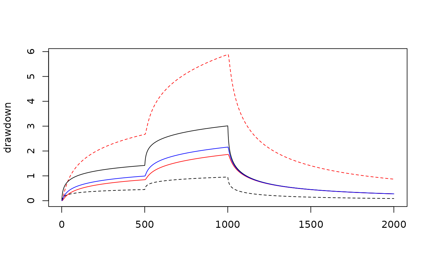
# Early time
plot(aquifer_theis_aniso~time, theis_aniso_iso_low,
     type = "l",
     ylab = "drawdown",
     xlab = "",
     lty = 2,
     xlim = c(0, 50),
     ylim = c(0, 1),
     col = "red")
points(aquifer_theis_aniso~time, theis_aniso_iso_high,
     type = "l",
     ylab = "drawdown",
     xlab = "",
     lty = 2)

points(aquifer_theis_aniso~time, theis_aniso_x,
     type = "l",
     ylab = "drawdown",
     xlab = "")
points(aquifer_theis_aniso~time, theis_aniso_y,
     type = "l",
     ylab = "drawdown",
     xlab = "",
     col = "red")
points(aquifer_theis_aniso~time, theis_aniso_xy,
     type = "l",
     ylab = "drawdown",
     xlab = "",
     col = "blue")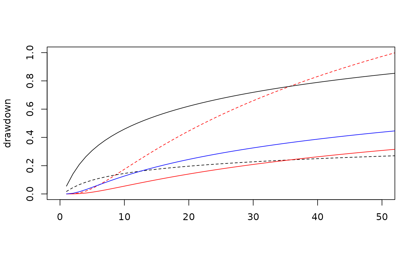
Hantush-Jacob leaky aquifer (Hantush-Jacob, 1955)
# high
hj <- recipe(formula = formula, data = dat) |>
  step_aquifer_leaky(time,
                     flow_rate,
                     leakage = 100,
                     radius = 100,
                     storativity = 1e-6,
                     transmissivity = 1e-4) |>
  plate()

plot(aquifer_leaky~time, hj, type = "l",
     ylab = "drawdown",
     xlab = "")
Barker-Herbert radially symmetric patch (Barker-Herbert, 1982)
Figure 2
formula <- as.formula(flow_rate~time)
q <- 0.05
t_1 <- 1.0
t_2 <- 1.0
s_1 <- 1e-5
s_2 <- 1e-7
r <- 10
R <- 100
time <- 10^seq(-4, 4, 0.01)
dat <- data.frame(time = time)

bh = recipe(formula = formula, data = dat) |>
  step_aquifer_patch(time = time,
                     flow_rate = q,
                     thickness = 1.0,
                     radius = r,
                     radius_patch = R,
                     specific_storage_inner = s_1,
                     specific_storage_outer = s_2,
                     hydraulic_conductivity_inner = t_1,
                     hydraulic_conductivity_outer = t_2,
                     n_stehfest = 12L) |>
  plate()

dim_time_scale = (4.0 * t_1) / (s_1 * r^2)
dim_s_scale = 4.0 * pi * t_1 / q
bh$dim_time <- bh$time * dim_time_scale
bh$dim_s <- bh$aquifer_patch * dim_s_scale

plot(dim_s~dim_time, bh, type = "l",
     ylab = "drawdown (dimensionless)",
     xlab = "time (dimensionless)",
     log = "x",
     ylim = c(0, 50))

bh = recipe(formula = formula, data = dat) |>
  step_aquifer_patch(time = time,
                     flow_rate = q,
                     thickness = 1.0,
                     radius = r,
                     radius_patch = R,
                     specific_storage_inner = s_1,
                     specific_storage_outer = s_2,
                     hydraulic_conductivity_inner = t_1,
                     hydraulic_conductivity_outer = t_2 * 10,
                     n_stehfest = 12L) |>
  plate()

dim_time_scale = (4.0 * t_1) / (s_1 * r^2)
dim_s_scale = 4.0 * pi * t_1 / q
bh$dim_time <- bh$time * dim_time_scale
bh$dim_s <- bh$aquifer_patch * dim_s_scale


points(dim_s~dim_time, bh, type = "l")

t_1 <- t_1 * 10.0
bh = recipe(formula = formula, data = dat) |>
  step_aquifer_patch(time = time,
                     flow_rate = q,
                     thickness = 1.0,
                     radius = r,
                     radius_patch = R,
                     specific_storage_inner = s_1,
                     specific_storage_outer = s_2,
                     hydraulic_conductivity_inner = t_1,
                     hydraulic_conductivity_outer = t_2,
                     n_stehfest = 12L) |>
  plate()

dim_time_scale = (4.0 * t_1) / (s_1 * r^2)
dim_s_scale = (4.0 * pi * t_1) / q
bh$dim_time <- bh$time * dim_time_scale
bh$dim_s <- bh$aquifer_patch * dim_s_scale


points(dim_s~dim_time, bh, type = "l")
Figure 3
formula <- as.formula(flow_rate~time)
t_1 <- 1.0
t_2 <- 1.0
s_1 <- 1e-5
s_2 <- 1e-5

bh = recipe(formula = formula, data = dat) |>
  step_aquifer_patch(time = time,
                     flow_rate = q,
                     thickness = 1.0,
                     radius = r,
                     radius_patch = R,
                     specific_storage_inner = s_1,
                     specific_storage_outer = s_2,
                     hydraulic_conductivity_inner = t_1,
                     hydraulic_conductivity_outer = t_2,
                     n_stehfest = 12L) |>
  plate()

dim_time_scale = (4.0 * t_1) / (s_1 * r^2)
dim_s_scale = 4.0 * pi * t_1 / q
bh$dim_time <- bh$time * dim_time_scale
bh$dim_s <- bh$aquifer_patch * dim_s_scale

plot(dim_s~dim_time, bh, type = "l",
     ylab = "drawdown (dimensionless)",
     xlab = "time (dimensionless)",
     log = "x",
     ylim = c(0, 50))

bh = recipe(formula = formula, data = dat) |>
  step_aquifer_patch(time = time,
                     flow_rate = q,
                     thickness = 1.0,
                     radius = r,
                     radius_patch = R,
                     specific_storage_inner = s_1,
                     specific_storage_outer = s_2,
                     hydraulic_conductivity_inner = t_1,
                     hydraulic_conductivity_outer = t_2 * 10,
                     n_stehfest = 12L) |>
  plate()

dim_time_scale = (4.0 * t_1) / (s_1 * r^2)
dim_s_scale = 4.0 * pi * t_1 / q
bh$dim_time <- bh$time * dim_time_scale
bh$dim_s <- bh$aquifer_patch * dim_s_scale


points(dim_s~dim_time, bh, type = "l")
t_1 <- t_1 * 10.0
bh = recipe(formula = formula, data = dat) |>
  step_aquifer_patch(time = time,
                     flow_rate = q,
                     thickness = 1.0,
                     radius = r,
                     radius_patch = R,
                     specific_storage_inner = s_1,
                     specific_storage_outer = s_2,
                     hydraulic_conductivity_inner = t_1,
                     hydraulic_conductivity_outer = t_2,
                     n_stehfest = 12L) |>
  plate()

dim_time_scale = (4.0 * t_1) / (s_1 * r^2)
dim_s_scale = (4.0 * pi * t_1) / q
bh$dim_time <- bh$time * dim_time_scale
bh$dim_s <- bh$aquifer_patch * dim_s_scale


points(dim_s~dim_time, bh, type = "l")
Figure 4
formula <- as.formula(flow_rate~time)
q <- 0.05
t_1 <- 1.0
t_2 <- 1.0
s_1 <- 1e-5
s_2 <- 1e-5
r <- 100
R <- 90

bh = recipe(formula = formula, data = dat) |>
  step_aquifer_patch(time = time,
                     flow_rate = q,
                     thickness = 1.0,
                     radius = r,
                     radius_patch = R,
                     specific_storage_inner = s_1,
                     specific_storage_outer = s_2,
                     hydraulic_conductivity_inner = t_1,
                     hydraulic_conductivity_outer = t_2,
                     n_stehfest = 14L) |>
  plate()

dim_time_scale = (4.0 * t_1) / (s_2 * r^2)
dim_s_scale = 4.0 * pi * t_2 / q
bh$dim_time <- bh$time * dim_time_scale
bh$dim_s <- bh$aquifer_patch * dim_s_scale

plot(dim_s~dim_time, bh, type = "l",
     ylab = "drawdown (dimensionless)",
     xlab = "time (dimensionless)",
     log = "x",
     ylim = c(0, 10))

bh = recipe(formula = formula, data = dat) |>
  step_aquifer_patch(time = time,
                     flow_rate = q,
                     thickness = 1.0,
                     radius = r,
                     radius_patch = R,
                     specific_storage_inner = s_1,
                     specific_storage_outer = s_2,
                     hydraulic_conductivity_inner = t_1,
                     hydraulic_conductivity_outer = t_2 * 10,
                     n_stehfest = 14L) |>
  plate()

dim_time_scale = (4.0 * t_2 * 10) / (s_1 * r^2)
dim_s_scale = 4.0 * pi * t_2 * 10 / q
bh$dim_time <- bh$time * dim_time_scale
bh$dim_s <- bh$aquifer_patch * dim_s_scale


points(dim_s~dim_time, bh, type = "l")

bh = recipe(formula = formula, data = dat) |>
  step_aquifer_patch(time = time,
                     flow_rate = q,
                     thickness = 1.0,
                     radius = r,
                     radius_patch = R,
                     specific_storage_inner = s_1,
                     specific_storage_outer = s_2,
                     hydraulic_conductivity_inner = t_1 * 10,
                     hydraulic_conductivity_outer = t_2,
                     n_stehfest = 14L) |>
  plate()

dim_time_scale = (4.0 * t_2) / (s_1 * r^2)
dim_s_scale = (4.0 * pi * t_2) / q
bh$dim_time <- bh$time * dim_time_scale
bh$dim_s <- bh$aquifer_patch * dim_s_scale


points(dim_s~dim_time, bh, type = "l")
Papadopulos-Cooper wellbore storage(Papadopulos-Cooper, 1967)
dat <- data.frame(time = 10^seq(-5, 2, length.out = 100),
                  flow_rate = rep(10.0, 100))
formula <- as.formula(flow_rate~time)

pc = recipe(formula = formula, data = dat) |>
  step_aquifer_wellbore_storage(time = time,
                                flow_rate = 10.0,
                                radius = 10.0,
                                radius_casing = 0.3,
                                radius_well = 0.3,
                                thickness = 1.0,
                                specific_storage = 1e-4,
                                hydraulic_conductivity = 1.0,
                                n_terms = 12L) |>
  plate()


th <- recipe(time~flow_rate, dat) |>
  step_aquifer_grf(time = time,
                   flow_rate = flow_rate,
                   thickness = 1.0,
                   radius = 10.0,
                   specific_storage = 1e-4,
                   hydraulic_conductivity = 1.0,
                   flow_dimension = 2.0) |>
  plate()
#> a: 0

plot(aquifer_wellbore_storage~time, pc,
     type = "l",
     log = "x",
     ylab = "drawdown",
     xlab = "elapsed time")
points(aquifer_grf~time, th, type = "l", col = "darkgrey", lty = "dashed")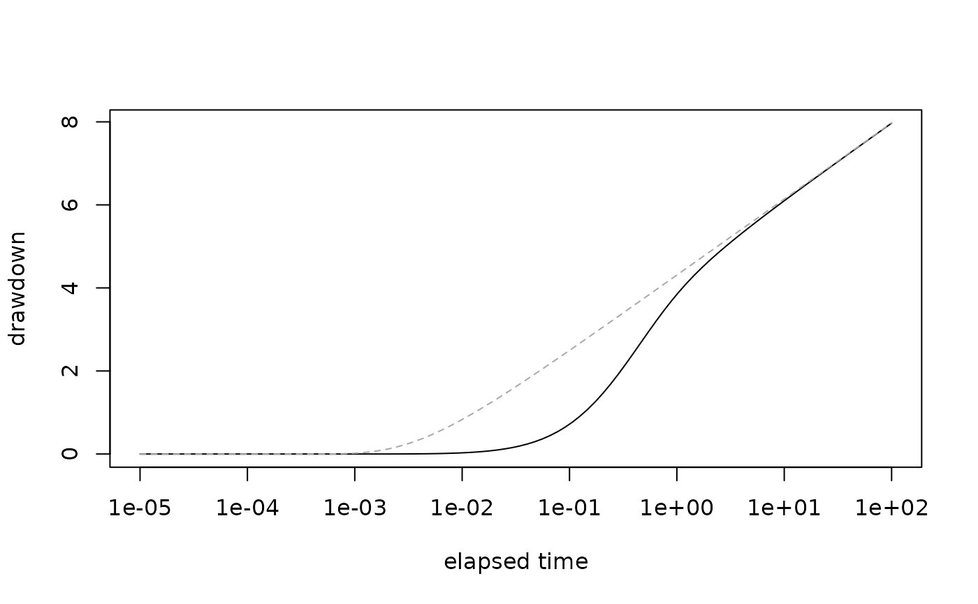
Jacob-Lohman constant drawdown (Jacob-Lohman, 1952)
time <- 10^seq(-5, 2, 0.1)
form <- formula(time~.)
dat <- data.frame(time = time)


jl = recipe(formula = form, data = dat) |>
  step_aquifer_constant_drawdown(time = time,
                                 drawdown = 10,
                                 thickness = 10,
                                 radius_well = 0.15,
                                 specific_storage = 1e-6,
                                 hydraulic_conductivity = 1) |>
  plate()

plot(aquifer_constant_drawdown~time, jl, type = "l",
     ylab = "flow rate",
     xlab = "elapsed time",
     log = "x")
References
Barker, J.A., A generalized radial flow model for hydraulic tests in fractured rock. Water Resour. Res., 24 (1988), pp. 1796-1804, 10.1029/WR024i010p01796
Barker, J.A., and R. Herbert, 1982: Pumping tests in patchy aquifers, Ground Water, vol. 20, No. 2, pp. 150-155.
Butler, J.J., 1988: Pumping tests in nonuniform aquifers – The radially symmetric case, Journal of Hydrology, Vol. 101, pp. 15-30.
Hantush, M.S. and C.E. Jacob, 1955. Non-steady radial flow in an infinite leaky aquifer, Am. Geophys. Union Trans., vol. 36, no. 1, pp. 95-100.
Heilweil, V.M. and Hsieh, P.A., 2006. Determining anisotropic transmissivity using a simplified Papadopulos method. Groundwater, 44(5), pp.749-753.
Jacob, C.E. and S.W. Lohman, 1952. Nonsteady flow to a well of constant drawdown in an extensive aquifer, Trans. Am. Geophys. Union, vol. 33, pp. 559-569.
Papadopulos, I.S., 1965. Nonsteady flow to a well in an infinite anisotropic aquifer.
Papadopulos, I.S. and H.H. Cooper, 1967. Drawdown in a well of large diameter, Water Resources Research, vol. 3, no. 1, pp. 241-244.
Prodanoff, J.H.A., Mansur, W.J. and Mascarenhas, F.C.B., 2006. Numerical evaluation of Theis and Hantush-Jacob well functions. Journal of hydrology, 318(1-4), pp.173-183.
sessionInfo()
#> R version 4.5.0 (2025-04-11)
#> Platform: x86_64-pc-linux-gnu
#> Running under: Ubuntu 24.04.2 LTS
#>
#> Matrix products: default
#> BLAS:   /usr/lib/x86_64-linux-gnu/openblas-pthread/libblas.so.3
#> LAPACK: /usr/lib/x86_64-linux-gnu/openblas-pthread/libopenblasp-r0.3.26.so;  LAPACK version 3.12.0
#>
#> locale:
#>  [1] LC_CTYPE=C.UTF-8       LC_NUMERIC=C           LC_TIME=C.UTF-8
#>  [4] LC_COLLATE=C.UTF-8     LC_MONETARY=C.UTF-8    LC_MESSAGES=C.UTF-8
#>  [7] LC_PAPER=C.UTF-8       LC_NAME=C              LC_ADDRESS=C
#> [10] LC_TELEPHONE=C         LC_MEASUREMENT=C.UTF-8 LC_IDENTIFICATION=C
#>
#> time zone: UTC
#> tzcode source: system (glibc)
#>
#> attached base packages:
#> [1] stats     graphics  grDevices utils     datasets  methods   base
#>
#> other attached packages:
#> [1] hydrorecipes_0.0.6 Bessel_0.6-1
#>
#> loaded via a namespace (and not attached):
#>  [1] gmp_0.7-5         plotly_4.10.4     sass_0.4.10       generics_0.1.3
#>  [5] tidyr_1.3.1       lattice_0.22-6    digest_0.6.37     magrittr_2.0.3
#>  [9] evaluate_1.0.3    grid_4.5.0        fastmap_1.2.0     jsonlite_2.0.0
#> [13] Matrix_1.7-3      httr_1.4.7        purrr_1.0.4       viridisLite_0.4.2
#> [17] scales_1.3.0      lazyeval_0.2.2    textshaping_1.0.0 jquerylib_0.1.4
#> [21] cli_3.6.5         RcppThread_2.2.0  Rmpfr_1.0-0       rlang_1.1.6
#> [25] munsell_0.5.1     cachem_1.1.0      yaml_2.3.10       tools_4.5.0
#> [29] parallel_4.5.0    dplyr_1.1.4       colorspace_2.1-1  ggplot2_3.5.2
#> [33] earthtide_0.1.7   vctrs_0.6.5       R6_2.6.1          lifecycle_1.0.4
#> [37] gslnls_1.4.1      fs_1.6.6          htmlwidgets_1.6.4 ragg_1.4.0
#> [41] pkgconfig_2.0.3   desc_1.4.3        pkgdown_2.1.1     bslib_0.9.0
#> [45] pillar_1.10.2     gtable_0.3.6      data.table_1.17.0 glue_1.8.0
#> [49] Rcpp_1.0.14       systemfonts_1.2.2 collapse_2.1.1    xfun_0.52
#> [53] tibble_3.2.1      tidyselect_1.2.1  knitr_1.50        htmltools_0.5.8.1
#> [57] rmarkdown_2.29    compiler_4.5.0