Barometric pressure steps
barometric_pressure.Rmd
# minute data
data(kennel_2020)
Time domain
Single value
- Clark’s 1967 method. Because Clark’s method is based on differences, the spacing between samples can affect the results. The following example uses differences of 1 minute, 1 hour, and 1 day for the Clark method.
- Least Squares method. The least squares method can be based on differenced or non-differenced data. In the following example the non-differenced data is used in addition to the 1 minute, 1 hour, and 1 day differences.
If the values vary based on the interval used in the difference calculation, it may suggest that the system does not behave like an ideal confined system or observational noise is high relative to true changes.
static_time <- recipe(wl~., kennel_2020) |>
  step_baro_clark(wl,
                  baro,
                  lag_space = 1,
                  inverse = FALSE) |> # 1 minutes (every minute differences)
  step_baro_clark(wl,
                  baro,
                  lag_space = 60,
                  inverse = FALSE) |> # 60 minutes (hourly differences)
  step_baro_clark(wl,
                  baro,
                  lag_space = 1440,
                  inverse = FALSE) |> # 1440 minutes (daily differences)
  step_baro_least_squares(wl, baro,
                          inverse = FALSE) |>
  step_baro_least_squares(wl, baro,
                          lag_space = 1L,
                          inverse = FALSE,
                          differences = TRUE) |> # 1 minutes (every minute differences)
  step_baro_least_squares(wl, baro,
                          lag_space = 60L,
                          inverse = FALSE,
                          differences = TRUE) |> # 60 minutes (hourly differences)
  step_baro_least_squares(wl, baro,
                          lag_space = 1440L,
                          inverse = FALSE,
                          differences = TRUE) |> # 1440 minutes (daily differences)
  prep() |>
  bake()

# The barometric efficiency is stored in the step (warning: this may change)
static_time$get_step_data("barometric_efficiency",
                          additional_columns = c("step_name",
                                                 "lag_space",
                                                 "differences"),
                          type = "dt")
#>           be               step_name lag_space differences
#>        <num>                  <char>     <num>      <lgcl>
#> 1: 0.1941766         step_baro_clark         1        TRUE
#> 2: 0.4738098         step_baro_clark        60        TRUE
#> 3: 0.8453437         step_baro_clark      1440        TRUE
#> 4: 0.8273019 step_baro_least_squares         1       FALSE
#> 5: 0.2493419 step_baro_least_squares         1        TRUE
#> 6: 0.4529153 step_baro_least_squares        60        TRUE
#> 7: 0.8410913 step_baro_least_squares      1440        TRUE
Response functions
Standard lags
formula <- as.formula(wl~.)

lag_standard <- recipe(formula = formula, data = kennel_2020) |>
  step_lead_lag(baro, lag = 0:1440) |>
  step_spline_b(datetime, df = 11, intercept = TRUE) |>
  step_drop_columns(c(baro, datetime, et)) |>
  step_ols(formula = formula) |>
  prep() |>
  bake()
resp_l <- lag_standard$get_response_data()
Distributed lags
lag_dl <- recipe(wl~., kennel_2020) |>
  step_distributed_lag(baro, knots = log_lags(15, 1440), intercept = TRUE) |>
  step_spline_b(datetime, df = 11, intercept = TRUE) |>
  step_drop_columns(c(baro, datetime, et)) |>
  step_ols(wl~.) |>
  prep() |>
  bake()
resp_dl <- lag_dl$get_response_data()
resp_dl <- lag_dl$get_step_data("response_data",
                                type = "dt")

plot(value~x, resp_l[resp_l$term == "lead_lag" & resp_l$variable == "cumulative", ],
     type = "l", ylim = c(0, 1),
     xlab = "Lag in minutes",
     ylab = "Cumulative Response"
     )
points(value~x, resp_dl[resp_dl$term == "distributed_lag_interpolated" & resp_dl$variable == "cumulative", ],
       type = "l", col = "red")
Frequency domain
Single value
These methods are based on the 2 cpd frequency which may not be indicative of the static barometric efficiency, in cases with a frequency dependent response (wellbore storage or non-confined conditions).
harmonic <- recipe(wl~., kennel_2020) |>
  step_baro_harmonic(datetime, wl, baro, et) |>
  prep() |>
  bake()

harmonic$get_step_data("barometric_efficiency")
#> [[1]]
#> [[1]]$ratio
#> [1] 0.5725228
#>
#> [[1]]$acworth
#> [1] 0.5940213
#>
#> [[1]]$rau
#> [1] 0.6108032
#>
#> [[1]]$tf
#> [1] 0.5844761
Transfer function
Three methods:
- pgram based
- assumes smooth periodogram
- Welch’s
- loss of low frequency information
- optimal values dependent on the subset length
- Experimental
- assumes smooth periodogram
- smoothing across multiple frequencies
- many higher frequecies discarded
- should be faster
- least squares fit of multiple frequencies
# this formula determines the variables to use for the transfer functions
formula_tf <- as.formula(wl ~ baro + et)

pg = recipe(wl~., data = kennel_2020) |>
  step_fft_transfer_welch(formula = formula_tf,
                          length_subset = 40000,
                          window = hydrorecipes:::window_rectangle(40000),
                          time_step = 60) |>
  step_fft_transfer_pgram(formula = formula_tf,
                          spans = c(3, 3),
                          time_step = 60) |>
  step_fft_transfer_experimental(formula = formula_tf,
                                 n_groups = 150,
                                 spans = c(3, 3),
                                 time_step = 60) |>
  prep("df") |>
  bake()

tf <- pg$get_transfer_data(type = "dt")

# plot the barometric transfer functions for the different methods
plot(Mod(value)~frequency,
     data = tf[grepl("fft_transfer_experimental", id) & variable == "wl_baro_et_1"],
     type = "l",
     log = "x",
     xlim = c(0.01, 200),
     ylim = c(0, 1),
     col = "#00900080")
#> Warning in xy.coords(x, y, xlabel, ylabel, log): 1 x value <= 0 omitted from
#> logarithmic plot
points(Mod(value)~frequency,
       data = tf[grepl("fft_transfer_welch", id) & variable == "wl_baro_et_1"],
       type = "l",
       col = "#90000050")
points(Mod(value)~frequency,
       tf[grepl("fft_transfer_pgram", id) & variable == "wl_baro_et_1"],
       type = "l",
       col = "#00009050")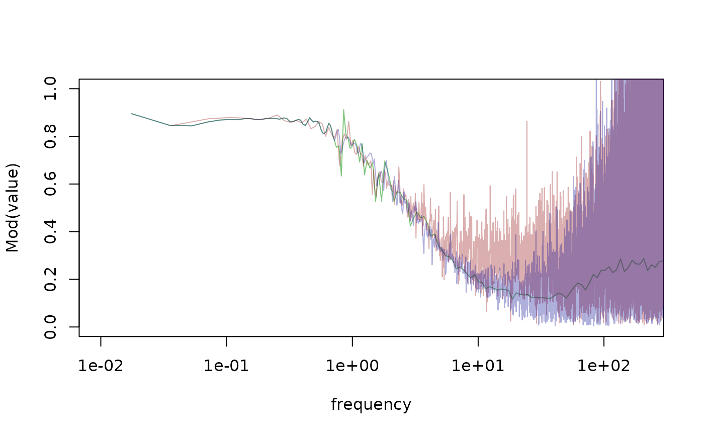
# plot the amplitude
plot(Mod(value)~frequency,
     data = tf[grepl("fft_transfer_experimental", id) & variable == "wl_baro_et_1"],
     type = "l",
     log = "x",
     xlim = c(0.01, 200),
     ylim = c(0, 1),
     col = "#00900080")
#> Warning in xy.coords(x, y, xlabel, ylabel, log): 1 x value <= 0 omitted from
#> logarithmic plot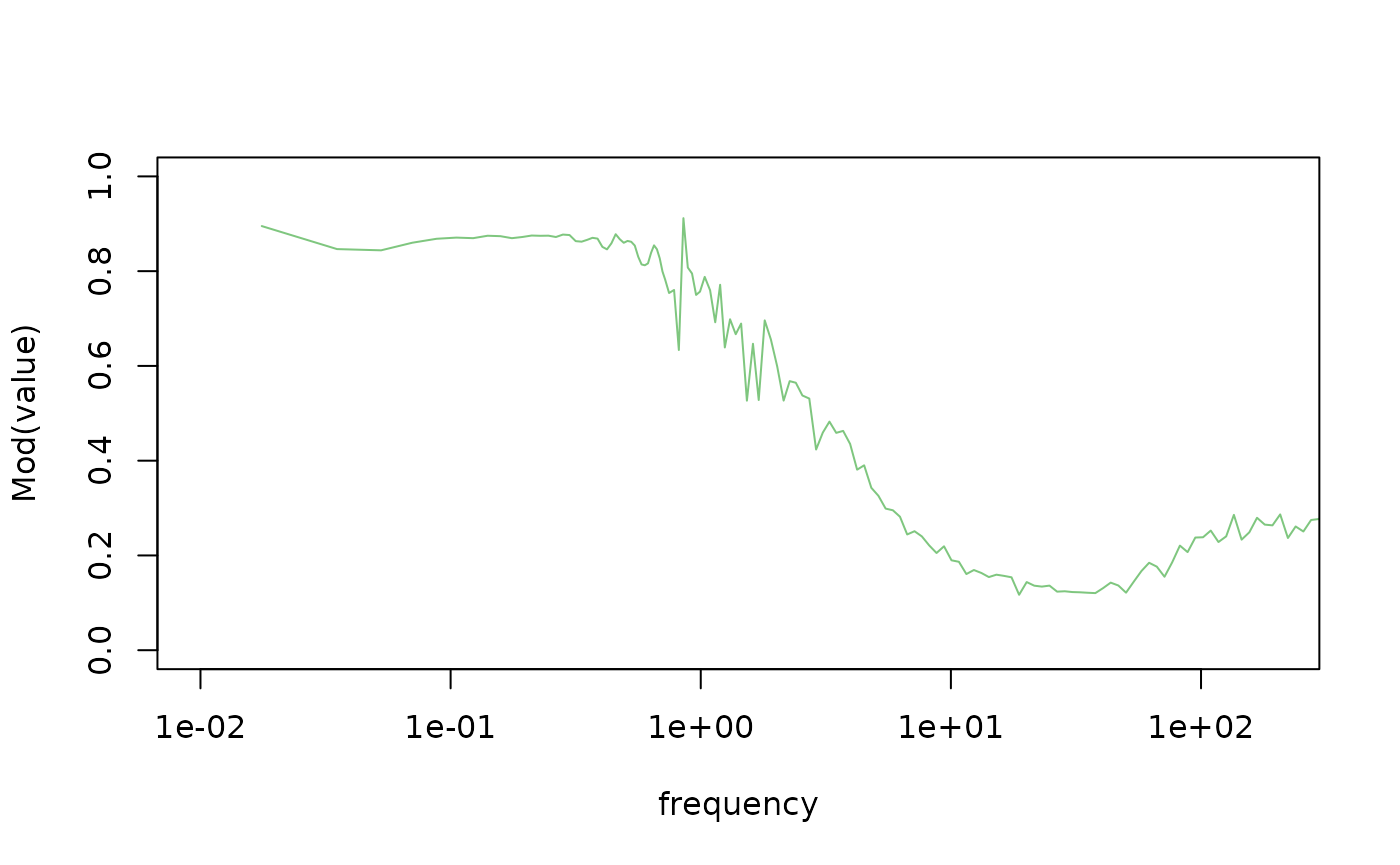
# plot the phase
plot(Arg(value)~frequency,
     data = tf[grepl("fft_transfer_experimental", id) & variable == "wl_baro_et_1"],
     type = "l",
     log = "x",
     xlim = c(0.01, 200),
     col = "#00900080")
#> Warning in xy.coords(x, y, xlabel, ylabel, log): 1 x value <= 0 omitted from
#> logarithmic plot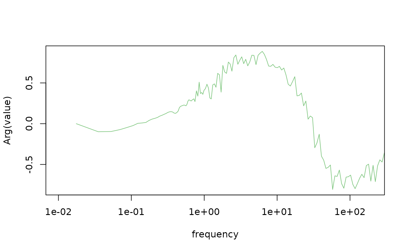
# tf <- pg$get_transfer_data(type = "dt")
# tmp <-  tf[grepl("fft_transfer_experimental", id) & variable == "wl_baro_et_1"]
# tmp[, frequency_log := log10(frequency)]
# tmp <- tmp[-c(1, .N)]
# fit_r <- lm(Re(value)~splines2::bSpline(frequency_log, df = 10), tmp)
# fit_i <- lm(Im(value)~splines2::bSpline(frequency_log, df = 10), tmp)
# plot(Re(value)~frequency_log, tmp)
# points(fit_r$fitted.values~frequency_log, tmp, type = "l", col = "red")
# plot(fit_r$fitted.values~frequency, tmp, type = "l", col = "red")
#
# plot(Im(value)~frequency_log, tmp)
# points(fit_i$fitted.values~frequency_log, tmp, type = "l", col = "red")
#
# plot(Im(value)~frequency, tmp)
# points(fit_i$fitted.values~frequency, tmp, type = "l", col = "red")
#
# brf_from_frf <- function(x) {
#
#   n <- floor(length(x) / 2) + 1
#
#   imp <- fft(x, inverse = TRUE) / length(x)
#   imp <- Mod(imp) * sign(Re(imp))
#
#   cumsum(rev(imp)[1:n] + (imp)[1:n])
#
# }
#
#
# x <- tmp$frequency
# y <- tmp$value
# frequency_to_time_domain <- function(x, y) {
#
#   dc1 <- y[1] # DC values
#   dc2 <- y[length(y)] # DC values
#   x_n <- x[-c(1, length(x))] # DC indices
#   y_n <- y[-c(1, length(y))] # DC values
#
#   # knots <- hydrorecipes:::log_lags(20, max(x_n))
#   # knots <- knots[-c(1, length(knots))]
#   # len <- min(knots):max(knots)
#   len <- seq(min(x_n), max(x_n), length.out = 10000)
# # this is used to smooth the complex response
#   sp_in  <- splines2::bSpline(x_n, df = 10)
#   sp_out <- splines2::bSpline(len, df = 10)
#
#
#     # out <- matrix(NA_real_,
#     #               nrow = length(len),
#     #               ncol = 1)
#     # out[1] <- len
#
# # loop through each transfer function - smooth the response - estimate brf
#     # for (i in 1:ncol(y_n)) {
#
# # smooth the real and imaginary components separately
#   re <- Re(y_n)
#   im <- Im(y_n)
#
#   fit_r <- RcppEigen::fastLm(X = sp_in, y = re)$coefficients
#   fit_i <- RcppEigen::fastLm(X = sp_in, y = im)$coefficients
#
#   re <- as.vector(sp_out %*% fit_r)
#   im <- as.vector(sp_out %*% fit_i)
#
# # estimate the brf from the smoothed uniform spaced frf
#         out <- brf_from_frf(complex(real = re, imaginary = im))
#     # }
#
#         plot(out, type = "l", log = "x")
#
#     out
# }
# tmp <- tf[grepl("fft_transfer_experimental", id) & variable == "wl_baro_et_1"]
# frequency_to_time_domain(x = tmp$frequency,
#                          y = tmp$value)
References
sessionInfo()
#> R version 4.5.0 (2025-04-11)
#> Platform: x86_64-pc-linux-gnu
#> Running under: Ubuntu 24.04.2 LTS
#>
#> Matrix products: default
#> BLAS:   /usr/lib/x86_64-linux-gnu/openblas-pthread/libblas.so.3
#> LAPACK: /usr/lib/x86_64-linux-gnu/openblas-pthread/libopenblasp-r0.3.26.so;  LAPACK version 3.12.0
#>
#> locale:
#>  [1] LC_CTYPE=C.UTF-8       LC_NUMERIC=C           LC_TIME=C.UTF-8
#>  [4] LC_COLLATE=C.UTF-8     LC_MONETARY=C.UTF-8    LC_MESSAGES=C.UTF-8
#>  [7] LC_PAPER=C.UTF-8       LC_NAME=C              LC_ADDRESS=C
#> [10] LC_TELEPHONE=C         LC_MEASUREMENT=C.UTF-8 LC_IDENTIFICATION=C
#>
#> time zone: UTC
#> tzcode source: system (glibc)
#>
#> attached base packages:
#> [1] stats     graphics  grDevices utils     datasets  methods   base
#>
#> other attached packages:
#> [1] hydrorecipes_0.0.6 Bessel_0.6-1
#>
#> loaded via a namespace (and not attached):
#>  [1] gmp_0.7-5         plotly_4.10.4     sass_0.4.10       generics_0.1.3
#>  [5] tidyr_1.3.1       lattice_0.22-6    digest_0.6.37     magrittr_2.0.3
#>  [9] evaluate_1.0.3    grid_4.5.0        fastmap_1.2.0     jsonlite_2.0.0
#> [13] Matrix_1.7-3      httr_1.4.7        purrr_1.0.4       viridisLite_0.4.2
#> [17] scales_1.3.0      lazyeval_0.2.2    textshaping_1.0.0 jquerylib_0.1.4
#> [21] cli_3.6.5         RcppThread_2.2.0  Rmpfr_1.0-0       rlang_1.1.6
#> [25] munsell_0.5.1     cachem_1.1.0      yaml_2.3.10       tools_4.5.0
#> [29] parallel_4.5.0    dplyr_1.1.4       colorspace_2.1-1  ggplot2_3.5.2
#> [33] earthtide_0.1.7   vctrs_0.6.5       R6_2.6.1          lifecycle_1.0.4
#> [37] gslnls_1.4.1      fs_1.6.6          htmlwidgets_1.6.4 ragg_1.4.0
#> [41] pkgconfig_2.0.3   desc_1.4.3        pkgdown_2.1.1     bslib_0.9.0
#> [45] pillar_1.10.2     gtable_0.3.6      data.table_1.17.0 glue_1.8.0
#> [49] Rcpp_1.0.14       systemfonts_1.2.2 collapse_2.1.1    xfun_0.52
#> [53] tibble_3.2.1      tidyselect_1.2.1  knitr_1.50        htmltools_0.5.8.1
#> [57] rmarkdown_2.29    compiler_4.5.0