Regression

library(hydrorecipes)
#> Loading required package: Bessel

This example generates the following regressor terms and then calculates the ordinary least squares solution.

• Distributed lag terms for barometric pressure
• B-spline terms for background trend
• Standard lagged terms for Earth tides
• Global intercept

The get_response_data function returns the response and cumulative responses based on the regression coefficients.

#|warning: false
#|message: false


library(hydrorecipes)
# kennel_2020 (1 minute interval)
#  water level
#  barometric pressure
#  synthetic earthtide
data(kennel_2020) 

form     <- as.formula(wl~.)
ba_knots <- log_lags(15, 1441)  # knots for distributed lag baro terms
df       <- 5                   # degrees of freedom for spline background trend

rec <- recipe(form, kennel_2020) |>
  step_distributed_lag(baro, knots = ba_knots) |>
  step_spline_b(datetime, df = df) |>
  step_lead_lag(et, lag = seq(-120, 120, 60)) |>
  step_intercept() |>
  step_drop_columns(c(baro, et, datetime)) |>
  step_ols(formula = form) |>
  prep() |>
  bake()


# responses
resp <- rec$get_response_data(type = "dt")

# barometric response function
plot(value~x, data = resp[term == "distributed_lag" & variable == "cumulative"], 
     type = "l",
     xlab = "Lag time in minutes",
     ylab = "Cumulative response")

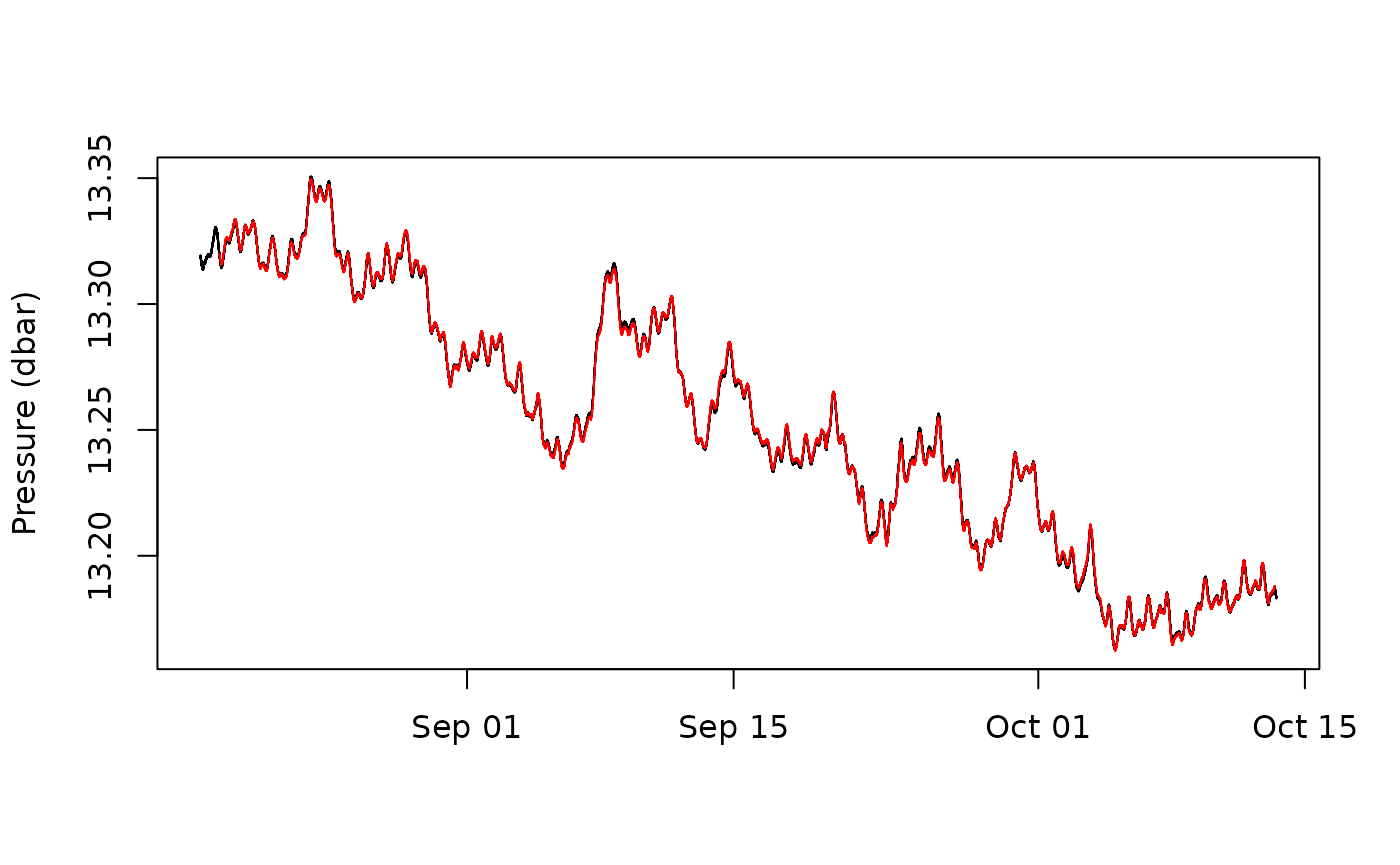
The regression coefficients can also be used to predict contributions from the regression model using the get_predict_data function. Summing all the terms give the predicted value from the regression model.

#|warning: false
#|message: false

# decomposition
pred <- cbind(kennel_2020, rec$get_predict_data())

# initial
plot(wl~datetime, pred, type = "l", 
       xlab = "", ylab = "Pressure (dbar)")

# predicted sum of components
points(wl_distributed_lag_baro + 
       wl_spline_b_datetime + 
       wl_lead_lag_et + 
       wl_intercept~datetime, pred, type = "l", col = "red")